Knowing how different market conditions affect the performance of your strategy can have a huge impact on your returns.

Certain strategies will perform well in highly volatile, choppy markets while others need a strong, smooth trend or they risk long periods of drawdown. Figuring out when you should start or stop trading a strategy, adjusting your risk and money management techniques, and even setting the parameters of your entry and exit conditions are all dependent on the market “regime”, or current conditions.

Being able to identify different market regimes and altering your strategy accordingly can mean the difference between success and failure in the markets. In this article we will explore how to identify different market regimes by using a powerful class of machine-learning algorithms known as “Hidden Markov Models.

Hidden Markov Models

Markov Models are a probabilistic process that look at the current state to predict the next state. A simple example involves looking at the weather. Let’s say we have three weather conditions (also known as “states” or “regimes”): rainy, cloudy, and sunny. If today is raining, a Markov Model looks for the probability of each different weather condition occurring. For example, there might be a higher probability that it will continue to rain tomorrow, a slightly lower probability that it will be cloudy, and a small probability that it will become sunny.

Today’s Weather	Tomorrow’s Weather	Probability of Change
Rainy	Rainy	65%
Rainy	Cloudy	25%
Rainy	Sunny	10%
Cloudy	Rainy	55%
Cloudy	Cloudy	20%
Cloudy	Sunny	25%
Sunny	Rainy	10%
Sunny	Cloudy	30%
Sunny	Sunny	60%

This seems like a very straightforward process but the complexity lies in not knowing the probability of each regime shift and how to account for these probabilities changing over time. This is where a Hidden Markov Model (HMM) comes into play. They are able to estimate the transition probabilities for each regime and then, based on current conditions, output the most probable regime.

The applications to trading are very clear. Instead of weather conditions, we could define the regimes as being bullish, bearish, or sideways markets, or high or low volatility, or some combination of factors that we know will have a large effect on the performance of our strategy.

Building a Model in R over Real Data

We are looking to find different market regimes based on these factors that we can then use to optimize our trading strategy. To do this, we’ll use the depmixS4 R library as well as EUR/USD day charts dating back to 2012 build the model.

First, let’s install the libraries and build our data set in R.

						install.packages(‘depmixS4’)

						library(‘depmixS4’) #the HMM library we’ll use
					

						install.packages(‘quantmod’)

						library(‘quantmod’) #a great library for technical analysis and working with time series
					

Load out data set (you can download it here), then turn it into a time series object.

						Date<-as.character(EURUSD1d[,1])

						DateTS<- as.POSIXlt(Date, format = "%Y.%m.%d %H:%M:%S") #create date and time objects

						TSData<-data.frame(EURUSD1d[,2:5],row.names=DateTS)

						TSData<-as.xts(TSData) #build our time series data set
					

						ATRindicator<-ATR(TSData[,2:4],n=14) #calculate the indicator

						ATR<-ATRindicator[,2] #grab just the ATR
					

						LogReturns <- log(EURUSD$Close) - log(EURUSD$Open) #calculate the logarithmic returns
					

						ModelData<-data.frame(LogReturns,ATR) #create the data frame for our HMM model
					

						ModelData<-ModelData[-c(1:14),] #remove the data where the indicators are being calculated
					

						colnames(ModelData)<-c("LogReturns","ATR") #name our columns
					

Now it's time to build the Hidden Markov Model!

						set.seed(1)

						HMM<-depmix(list(LogReturns~1,ATR~1),data=ModelData,nstates=3,family=list(gaussian(),gaussian())) #We’re setting the LogReturns and ATR as our response variables, using the data frame we just built, want to set 3 different regimes, and setting the response distributions to be gaussian.
					

						HMMfit<-fit(HMM, verbose = FALSE) #fit our model to the data set
					

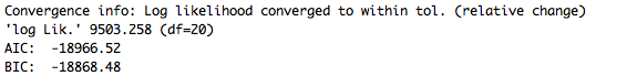
						print(HMMfit) #we can compare the log Likelihood as well as the AIC and BIC values to help choose our model
					

						summary(HMMfit)
					

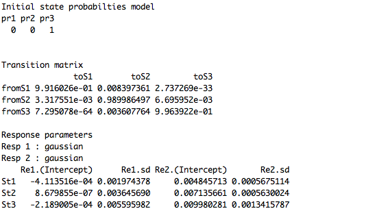
The transition matrix gives the us probability of moving from one state to the next.

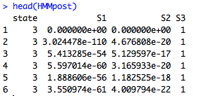
						HMMpost<-posterior(HMMfit) #find the posterior odds for each state over our data set
					

						head(HMMpost) #we can see that we now have the probability for each state for everyday as well as the highest probability class. 
					

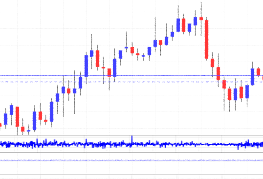
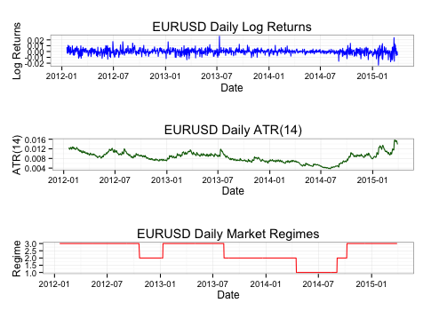
Let’s see what we found:

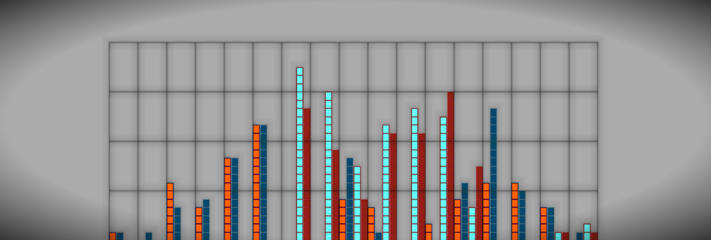
The probability of each regime separately:

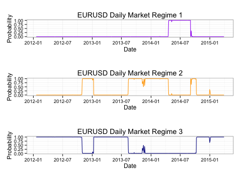
What we can see is that regime 3 tends to be times of high volatility and large magnitude moves, regime 2 is characterized by medium volatility, and regime 1 consists of low volatility.

Applications to Your Strategy

There are multiple different ways of applying HMM to your trading. The simplest would be to see if there is a relationship between the regime and performance of your strategy, allowing you to adjust accordingly. You could also adjust the parameters of your strategy based on the regime. For example, larger take profits and stop losses in times of high volatility. There is also the option of creating unique strategies for different regimes.

Hidden Markov Models are powerful tools that can give you insight into changing market conditions. They have a wide range of applications that can allow you to greatly improve the performance of your strategy.

Take a look at TRAIDE for other ways to apply machine learning to your trading!

Happy TRAIDING!