In our last article we went through a basic example of building a machine-learning algorithm to predict the direction of Apple stock, now we’ll explore how you can actually use these algorithms to help you come up with your own strategy.

Let’s say you like to use a variety of technical indicators and you want to create a strategy that looks for specific high-probability trading opportunities. For example, what if an RSI value above 85 AND a MACD signal line under 20 is a great opportunity to go short? You can either spend days/weeks/months trying to discover those relationships on your own or use a decision tree, a powerful and easily interpretable algorithm, to give you a huge head start.

Lets first gain a basic understanding of how decision trees work then step through an example of how we can use them to quickly and easily build a strategy to trade Bank of America stock.

How a Decision Tree Works

Decision trees are one of the more popular machine-learning algorithms for their ability to model noisy data, easily pick up non-linear trends, and capture relationships between your indicators; they also have the benefit of being easy to interpret. Decision trees take a top-down, “divide-and-conquer” approach to analyzing data. They look for the indicator, and indicator value, that best splits the data into two distinct groups. The algorithm then repeats this process on each subsequent group until it correctly classifies every data point or a stopping criteria is reached. Each split, known as a “node”, tries to maximize the purity of the resulting “branches”. The purity is basically the probability that a data point falls in a given class, in our case “up” or “down”, and is measured by the “information gain” of each split.

Decision trees, however, can easily overfit the data and perform poorly when looking at new data. There are generally three ways to address this issue:

• You can control the growth of the tree by specifying either a threshold on the information gain or a minimum number of data points in each branch to justify a split. This creates a tree that will attempt to capture larger, more broad patterns and not focus on minor splits that may be unique to your particular data set.


• You can also prune back the tree after it has already been built. Usually this is done by selecting the tree size that minimizes the cross-validated error. Cross-validation is a process that partitions the data into multiple sections then uses all but one section to build the model and the remaining section to test the model. This process is then repeated, using each section to test the model, and the tree size with the lowest average error is chosen. This is also a great way to reduce overfitting if you have limited data.


• A more sophisticated approach is to build many different trees and use them collectively to make predictions. There are three popular techniques, bagging, boosting, and random forests, that we will cover in a later article.

Now that we have a basic understanding of how decision trees work, let’s build our strategy!

Building a Strategy

Let’s see how we can quickly build a strategy using 4 technical indicators to see whether today’s price of BoA’s stock is going to close up or down.

First, let’s make sure we have all the libraries we need installed and loaded.

						install.packages("quantmod")


						library("quantmod")


						#Allows us to import the data we need and calculate the technical indicators

					

						install.packages("rpart") 


						library("rpart")


						#Gives us access to the decision trees we will be using. (I had to update my version of R in order to install this one.)

					

						install.packages("rpart.plot")


						library("rpart.plot")


						#Let’s us easily create good looking diagrams of the trees.

					

Next, let’s grab all the data we will need and calculate the indicators.

						startDate = as.Date("2012-01-01")


						#The beginning of the date range we want to look at

					

						endDate = as.Date("2014-01-01")


						#The end of the date range we want to look at

					

						getSymbols("BAC", src = "yahoo", from = startDate, to = endDate) 


						#Retrieving the daily OHLCV of Bank of America’s stock from Yahoo Finance

					

						RSI3<-RSI(Op(BAC), n= 3)


						#Calculate a 3-period relative strength index (RSI) off the open price

					

						EMA5<-EMA(Op(BAC),n=5)


						#Calculate a 5-period exponential moving average (EMA)


						EMAcross<- Op(BAC)-EMA5


						#Let’s explore the difference between the open price and our 5-period EMA

					

						MACD<-MACD(Op(BAC),fast = 12, slow = 26, signal = 9)


						#Calculate a MACD with standard parameters


						MACDsignal<-MACD[,2]


						#Grab just the signal line to use as our indicator.

					

						SMI<-SMI(Op(BAC),n=13,slow=25,fast=2,signal=9) 


						#Stochastic Oscillator with standard parameters


						SMI<-SMI[,1]


						#Grab just the oscillator to use as our indicator

					

Then calculate the variable we are looking to predict and build our data sets.

						PriceChange<- Cl(BAC) - Op(BAC)


						#Calculate the difference between the close price and open price


						Class<-ifelse(PriceChange>0,"UP","DOWN")


						#Create a binary classification variable, the variable we are trying to predict.

					

						DataSet<-data.frame(RSI3,EMAcross,MACDsignal,SMI,Class)


						#Create our data set


						colnames(DataSet)<-c("RSI3","EMAcross","MACDsignal","Stochastic","Class") 


						#Name the columns


						DataSet<-DataSet[-c(1:33),]


						#Get rid of the data where the indicators are being calculated

					

						TrainingSet<-DataSet[1:312,]


						#Use 2/3 of the data to build the tree


						TestSet<-DataSet[313:469,]


						#And leave out 1/3 data to test our strategy

					

Now that we have everything we need, let’s build that tree!

						DecisionTree<-rpart(Class~RSI3+EMAcross+MACDsignal+Stochastic,data=TrainingSet, cp=.001)


						#Specifying the indicators to we want to use to predict the class and  controlling the growth of the tree by setting the minimum amount of information gained (cp) needed to justify a split.

					

Great! We have our first decision tree, now let’s see what we built.

						prp(DecisionTree,type=2,extra=8)


						#Nice plotting tool with a couple parameters to make it look good. If you want to play around with the visualization yourself,  here is a great resource.

					

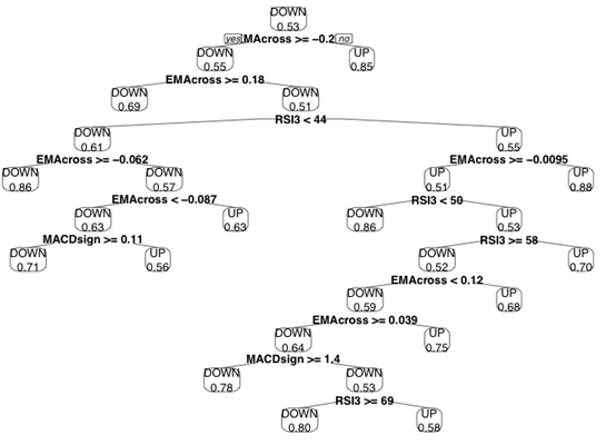A quick note on interpreting the tree: The nodes represent a split, with the left branch reflecting a “yes” answer and the right branch a “no”. The number in the final “leaf” is the percentage of instances that were corrected classified by that node.

Decision trees can also be used to help select and evaluate indicators. Indicators that are closer to the top of the tree lead to more pure splits, and contain more information, than those towards the bottom of the tree. In our case, the Stochastic Oscillator didn’t even make it onto the tree!

While you now have a set a rules to follow, we are going to want to make sure that we aren’t overfitting the data, so let’s prune the tree. An easy way to do this is by looking at the complexity parameter, which is basically the “cost”, or decrease in performance, of adding another split, and choose the tree size that minimizes our cross-validated error.

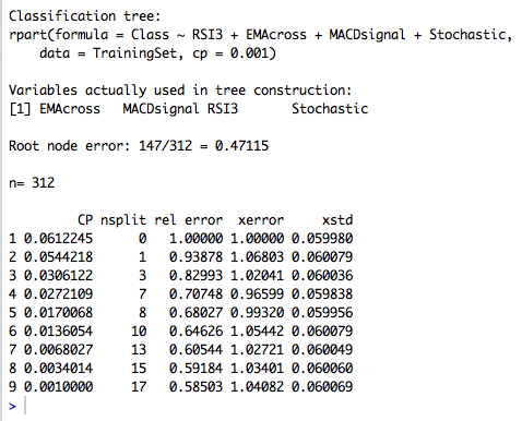
						printcp(DecisionTree)


						#shows the minimal cp for each trees of each size.


						plotcp(DecisionTree,upper="splits")


						#plots the average geometric mean for trees of each size.


					

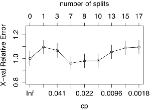
You can see that our tree is actually best off with just 7 splits! (Due to cross-validation process that randomly segments the data to test the model, you may get slightly different results than what you see here. One of the drawbacks of decision trees is that they can be “unstable”, meaning that small changes in the data can lead to large differences in the tree. That’s why the pruning process, and other ways to decrease overfitting, are so important.)

Let’s prune back that tree and see what our newly-pruned strategy looks like.

						PrunedDecisionTree<-prune(DecisionTree,cp=0.0272109)


						#I am selecting the complexity parameter (cp) that has the lowest cross-validated error (xerror)

					

Now let’s take a look at the freshly-pruned tree.

						prp(PrunedDecisionTree, type=2, extra=8)


					

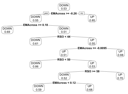Much more manageable! And we see that the MACDsignal line is no longer included! After starting out with 4 indicators, we see that only a 3-period RSI and the difference between the price and a 5-period EMA are actually important when looking to predict whether the day’s price will close up or down.

Time to see how well it does over our test set.

						table(predict(PrunedDecisionTree,TestSet,type="class"),TestSet[,5],dnn=list('predicted','actual'))


					

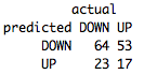
Overall, not bad; it was about 52% accurate. More importantly, you have the basis of strategy with clearly-defined, mathematically-supported parameters! With only about 25 commands, we were able to learn about which indicators were important and what specific conditions we should be looking for to make a trade. Now you can take these rules and apply them to your own trading or work on improving the tree.

In our next article, we will look into using another powerful machine-learning algorithm, a support vector machine, and how we can transform its findings into an even more robust strategy!

Happy trading! If you haven't already, sign up for TRAIDE. You will be able to go through the same process with a variety of algorithms, in an interactive interface, without a single line of code.