Once you have built a model, you need to make sure it is robust and going to give you profitable signals when you trade live.

In this post, we are going to go over 3 easy ways you can improve the performance of your model.

Before you can improve your model, you must be able to establish a baseline performance to then improve upon. One great way to do this is by testing it over new data. However, even in the data-rich financial world, there is a limited amount of data and so you must be very careful about how you use it. For this reason, it is best to split your data set into three distinct parts.

• Training Set:
  • This is the data that you use to train, or build, the model. The algorithm will attempt to find relationships between your inputs (our indicators) and the output (whether the next day’s price will close up or down). Usually you want to reserve around 60% of your data for the training.
• Test Set:
  • We will use the test set to evaluate the model’s performance over data that wasn’t used to build it. This is the set that we will use to compare different models so it is important that it is representative of the data set as a whole. Generally, about 20% of the data should be set aside for the test set.
• Validation Set:
  • The validation set is used to measure how well our final model will perform moving forward. You can only use this data once for it to be truly “out-of-sample” or else you are merely overfitting a model to this final data set. If the results aren’t up to your standards, you have to start back at square one using a different validation set in order to be confident you have built a robust model. The final 20% of the data is usually reserved as your validation set.

1. Understanding Your Model

Before you can improve your model, you need to understand the characteristics of your model; specifically, where does it fall in the bias-variance tradeoff? Bia, also known as underfitting, is caused by the model making overly simplistic assumptions of the data. Variance, on the other hand, is what we know as overfitting, or merely modeling the inherent noise in your data. The trick is to capture as much of the underlying signal in your data without fitting to the random noise.

An easy way to know where your model falls in the bias-variance tradeoff is comparing the error on your training set to your test set error. If you have a high training set error and a high test set error, you are most likely have a high bias, whereas if you have a low training set error and a high test set error, you are suffering from high variance.

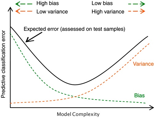
You tend to get better results over new data if you err on the side of underfitting, but here are a couple ways to address both issues:

High Variance (Overfitting)	High Bias (Underfitting)
Use more data	Add more inputs
Regularization*	Create more sophisticated features
Ensemble: bagging	Ensemble: boosting

*Regularization is a process that penalizes models for becoming more complex and places a premium on simpler models (You can find more information and an example in R here.

Now that we understand where our model falls on the bias-variance tradeoff, let’s explore other ways to improve our model.

2. Feature Creation

Like we covered in a previous article, choosing the inputs to your model are incredible important. The mantra “garbage in garbage out” is very applicable, where if we are not giving valuable information to the algorithm, it is not going to be able to find any useful patterns or relationships.

While you might say “I use a 14-period RSI to trade”, there is actually a lot more that goes into it. You are most likely also incorporating the slope of the RSI, whether it is at a local maximum or minimum, incorporating divergence from the price, and numerous other factors. However, the model receives only one piece of information: the current value of the RSI. By creating a feature, or a calculation derived from the value of the RSI, we are able to provide the algorithm with much more information in a single value.

Let’s use a Naive Bayes algorithm, a more stable algorithm that tends to have a high bias, to see how creating more sophisticated features can improve its performance. To learn more about decision trees, be sure to take a look at my previous post on how to use a decision tree to trade Bank of America stock..

First, let’s install the packages we need, get our data set up and calculate the baseline inputs.

						install.packages(“quantmod”)

						library(quantmod)

						install.packages(“e1071”)

						library(e1071)

					

						startDate = as.Date("2009-01-01")

						endDate = as.Date("2014-06-01")

						#Set the date range we want to explore
					

						getSymbols("MSFT", src = "yahoo", from = startDate, to = endDate)

						#Grab our data
					

						EMA5<-EMA(Op(MSFT),5)

						RSI14<-RSI(Op(MSFT),14)

						Volume<-lag(MSFT[,5],1)

						#Calculate our basic indicators. Note: we have to lag the volume to use yesterday’s volume as an input to avoid data snooping, whereas we avoid that problem by calculating the indicators off the open price
					

						PriceChange<- Cl(MSFT) - Op(MSFT)

						Class<-ifelse(PriceChange>0,"UP","DOWN")

						#Create the variable we are looking to predict
					

						BaselineDataSet<-data.frame(EMA5,RSI14,Volume)

						BaselineDataSet<-round(BaselineDataSet,2)

						#Like we mentioned in our previous article, we need to round the inputs to two decimal places when using a Naive Bayes algorithm
					

						BaselineDataSet<-data.frame(BaselineDataSet,Class)

						BaselineDataSet<-BaselineDataSet[-c(1:14),]

						colnames(BaselineDataSet)<-c("EMA5","RSI14","Volume","Class")

						#Create our data set, delete the periods where our indicators are being calculated and name the columns
					

						BaselineTrainingSet<-BaselineDataSet[1:808,];BaselineTestSet<-BaselineDataSet[809:1077,];BaselineValSet<-BaselineDataSet[1078:1347,]

						#Divide the data into 60% training set, 20% test set, and 20% validation set
					

And then build our baseline model.

 
						BaselineNB<-naiveBayes(Class~EMA5+RSI14+Volume,data=BaselineTrainingSet)

					

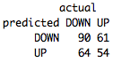
						table(predict(BaselineNB,BaselineTestSet),BaselineTestSet[,4],dnn=list('predicted','actual')) 
					

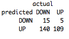Not great. Only 46% accurate and we have a fairly strong upward bias. This is a strong sign that our model isn’t sufficiently complex enough to model our data and is underfitting.

Now, let’s create some more sophisticated features and see if we are able to reduce this bias.

						EMA5Cross<-EMA5-Op(MSFT)

						RSI14ROC3<-ROC(RSI14,3,type="discrete")

						VolumeROC1<-ROC(Volume,1,type="discrete")

						#Let’s explore the distance between our 5-period EMA and the open price, and the one and three period rate of changes (ROC) of our RSI and Volume, respectively
					

						FeatureDataSet<-data.frame(EMA5Cross,RSI14ROC3,VolumeROC1)

						FeatureDataSet<-round(FeatureDataSet,2)

						#Round the indicator values
					

						FeatureDataSet<-data.frame(FeatureDataSet, Class)

						FeatureDataSet<-FeatureDataSet[-c(1:17),]

						colnames(FeatureDataSet)<-c("EMA5Cross","RSI14ROC3","VolumeROC1","Class")

						#Create and name the data set
					

						FeatureTrainingSet<-FeatureDataSet[1:806,]; FeatureTestSet<-FeatureDataSet[807:1075,]; FeatureValSet<-FeatureDataSet[1076:1344,]

						#Build our training, test, and validation sets

					

And finally build our new model.

						FeatureNB<-naiveBayes(Class~EMA5Cross+RSI14ROC3+VolumeROC1,data=FeatureTrainingSet)

					

Let’s see if we were able to reduce the bias of our model.

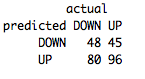
						table(predict(FeatureNB,FeatureTestSet),FeatureTestSet[,4],dnn=list('predicted','actual'))
					

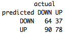We were able to improve the accuracy by 7% up to 53% with only fairly basic features! By exploring how you actually look at your indicators and translating that into a value the model can understand, you should be able to improve the performance even more!

3. Ensemble Techniques

One of the most powerful methods of improving the performance of your model is to actually incorporate multiple models into what is known as an “ensemble”. The theory is that by combining multiple models and aggregating their predictions, we are able to get much more robust results. Empirical tests have shown that even ensembles of basic models are able to outperform much more powerful individual models.

There are three basic ensemble techniques:

• Bagging:
  • Bagging works by building models based off slightly different training sets and averaging their results to get a single prediction. The training set is altered by replicating or deleting data points, resulting in slightly different models. This process works well with unstable models (like decision trees) or if there is a degree of randomness in the model building process (like the initial weights of a neural network). By taking the average prediction of the collection of models with high variance, we are able to decrease the overall variance without increasing the bias, which can lead to better results.
• Boosting:
  • Boosting works in an iterative fashion by encouraging models to become experts where earlier models were weak. Greater weights on previously incorrectly classified data points and the final prediction is made by combining a weighted vote of all the models in the ensemble. This technique works well with “weak” classifiers that tend to underfit the data, like simple decision trees or Naive Bayes classifiers. Here we are using models with a high bias to focus on subsets of the data, allowing the ensemble as a whole to capture more of the underlying signal.
• Stacking:
  • So far we have only explored ensembles containing models with the same underlying algorithm, but what if we have multiple models based on different algorithms? Stacking incorporates a wide variety of models by using a “meta learner” to try to figure out the best combination of individual models. Predictions made by each individual model are then fed into the “meta learner”, which analyzes the characteristics of each model and outputs the final prediction. Stacking is best used when you have a collection of models built off different underlying learning algorithms.

Let’s use a model with high variance, an unpruned decision tree, to show how bagging can improve its performance.

First, we’ll build a decision tree using the same features we constructed for the Naive Bayes.

						install.packages(“rpart”)

						library(rpart)

						install.packages(“foreach”)

						library(foreach)
					

						BaselineDecisionTree<-rpart(Class~EMA5Cross+RSI14ROC3+VolumeROC1,data=FeatureTrainingSet, cp=.001)
					

And see how well it does over the test set.

						table(predict(BaselineDecisionTree,FeatureTestSet,type="class"),FeatureTestSet[,4],dnn=list('predicted','actual'))
					

Right around 51%. Comparing that to the accuracy on our training set, which was 73%, we can see our unpruned decision tree is greatly overfitting the training set.

Now let’s see if a bagging ensemble can help reduce that. While R provides a couple different bagging algorithms, let’s build an algorithm ourselves so we can have more control over the underlying algorithm and the bagging parameters.

						length_divisor<-10

						iterations<-1501

						#This determines how we create subsets of the training set and how many models to include in the ensemble. Here we are building 1501 different models off a randomly sampled 1/10th of the data 
					

						 BaggedDecisionTree<- foreach(m=1:iterations,.combine=cbind) %do% {
						 training_positions <- sample(nrow(FeatureTrainingSet), size=floor((nrow(FeatureTrainingSet)/length_divisor)))

						 train_pos<-1:nrow(FeatureTrainingSet) %in% training_positions
						

						BaselineDecisionTree<-rpart(Class~EMA5Cross+RSI14ROC3+VolumeROC1,data=FeatureTrainingSet[train_pos,])

						 predict(BaselineDecisionTree,newdata=FeatureTestSet)

							}

						#This is our handmade bagging algorithm. Thanks to Vic Paruchuri for this.
					

						CumulativePredictions<-apply(BaggedDecisionTree[,1:iterations],1,function(x){s<-(sum(x)/iterations)

						round(s,0)})

						#Now we need to aggregate the predictions of our 1501 decision trees
					

						FinalPredictions<-ifelse(CumulativePredictions==1,"DOWN","UP")

						#Return from a binary output to our classification labels
					

Once again, let’s evaluate our performance over the test set. (Since the tree is built from random subsets of the training set, you may get slightly different results; this is one of downsides of working with unstable algorithms like decision trees.)

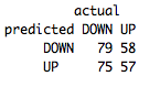
						table(FinalPredictions,FeatureTestSet[,4],dnn=list('predicted','actual'))
					

Much better! By decreasing the variance, we were able to increase our performane to 54%.

Finally, let's take our best model, and run it over our validation set to make sure that we have built a robust model.

While the bagged decision tree and Naive Bayes model performed similarly, I like to err on the side of the model with high bias rather than high variance. Models that tend to underfit the data may not perform as well over your training and test set, but you can be more confident that they will perform about the same over new data. Models with a high variance, on the other hand, run a much greater risk of performing significantly worse when using unseen data.

For that reason, let’s go with our Feature Naive Bayes as our final model.

And now to test it over the validation set:

(Fingers crossed…..)

						table(predict(FeatureNB,FeatureValSet),FeatureValSet[,4],dnn=list('predicted','actual'))
					

Not bad at all and very consistent with our training and test error! Our final accuracy over the validation set was 54%. Looks like we have built a fairly robust model!

Conclusion

The first step to improving the performance of your model is to understand where it falls on the bias-variance tradeoff. Only once you are able to diagnose your model can you then prescribe the necessary treatments.

With TRAIDE, you will be able to not only quickly evaluate your model but also easily implement the techniques included in this article and more to improve its performance. Pre-register here to add these machine-learning techniques to your arsenal!

In our next article, we will explore how you can derive your own trading rules from these type of models.

Happy trading!